
IMDB Web Scrape and Model
Objective:
What makes for a good movie? In this short project, we will scrape data from the IMDB list of most popular movies from 2018 to see what movie traits and characteristics correlate with movie quality. As a measure of quality, we will use IMDB user score ratings for each movie, which are measured as a score out of 10.
Analysis:
First, I will load the required packages and scrape the data from IMDB.
library(rvest)
library(R.utils)
library(ggplot2)
library(betareg)
library(lmtest)

# Specifying the url for desired website to be scraped
url <- 'https://www.imdb.com/search/title?title_type=feature&release_date=2018-01-01,2018-12-31&count=100&view=advanced'

# Reading the HTML code from the website
webpage <- read_html(url)

# Scraping desired fields
genre <- html_nodes(webpage, '.genre')
runtime <- html_nodes(webpage, '.runtime')
critic_score <- html_nodes(webpage, '.ratings-metascore')
gross <- html_nodes(webpage, 'span')
user_score <- html_nodes(webpage, 'strong')

# Converting the data to text to make it easier to work with
genre_data <- html_text(genre)
runtime_data <- html_text(runtime)
critic_score_data <- html_text(critic_score)
gross_data <- html_text(gross)
user_score_data <- html_text(user_score)
Now we will need to clean our data to make it useable for our model.
I will start out by cleaning out the extra characters from the genre variable. Many movies have multiple genre tags. For simplicity, I will categorize them using only the main genre tag that appears first in the list.
genre_data = sub("\\,.*", "", substring(genre_data, 2))
genre_data = gsub(" ", "", genre_data, fixed = TRUE)
# some genres only appear a few times. We'll group these together as "other"
filter_cats = function(v, top, other = 'other'){
  cv = class(v)
  v = as.character(v)
  v[factor(v, levels = top) %>% is.na()] = other
  if(cv == 'factor') v = factor(v, levels = c(top, other))
  v
}
new_genre_data = filter_cats(genre_data,
                             c("Action", "Adventure", "Biography", "Comedy", "Drama"),
                             "Other")
new_genre_data = as.factor(new_genre_data)
We will do the same with the runtime variable now and remove extra characters.
new_runtime_data = gsub(" ", "", substring(runtime_data, 1,3), fixed = TRUE)
new_runtime_data = as.numeric(new_runtime_data)
Next I will clean the critic score variable. Some movies don’t have a score, so we’ll fill these in with the mean.
This is not a great assumption because missing ratings likely occur non-randomly; for example, less popular movies may be less likely to be rated by critics, and also more likely to be of below average quality.
Despite this potential bias, only a few movies have this information missing so this will do for now. Many of these observations with missing values will be filtered out in the next few steps anyway, so using the mean for missing variables is unlikely to change our end result.
new_critic_score = substring(critic_score_data, 2,4)
new_critic_score = gsub(" ", "", new_critic_score, fixed = TRUE)
new_critic_score = as.numeric(new_critic_score)
m = mean(new_critic_score)
for(i in c(31, 55, 69, 85, 89)){
  new_critic_score = insert(new_critic_score, i,
                            values=m, useNames=TRUE)
}
Next, clean the extra text from the gross variable. This variable measures gross income in millions of dollars. Some observations are missing information for this variable, likely because they are Netflix exclusives or TV seasons. We’ll limit our analysis to movies that played in theaters by filtering these out.
filter_gross = grep("$", gross_data, fixed = TRUE)
new_gross = transform(filter_gross, gross_data = regmatches(gross_data,
                                              regexpr("(?<=[$])\\w+", gross_data, perl = TRUE)))
new_gross_data = as.character(new_gross$gross_data)
# Identify the missing values so they can be filtered out
for(i in c(8,10,31,48,55,58,59,69,77,79,80,85,89,93)){
  new_gross_data = insert(new_gross_data, i,
                            values="Missing", useNames=TRUE)
}
Clean the user score and convert it to a numeric variable.
new_user_score = user_score_data[7:106]
new_user_score = as.numeric(new_user_score)
Since these scores are bounded between 1 and 10, OLS is not our best option. Instead, let’s divide scores by 10 and use the beta regression model introduced by Ferrari and Cribari-Neto (2004). We’ll scale critic score to between 0 and 1 as well, just to make comparisons easier.
adj_user_score = new_user_score/10
adj_critic_score = new_critic_score/100
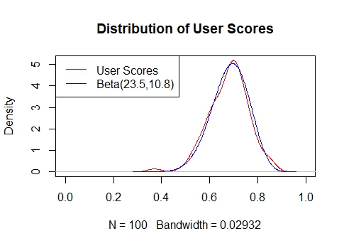
The user scores now roughly follow a beta distribution.
plot(density(adj_user_score), col = 'red', main = "Distribution of User Scores", xlim=c(0,1))
lines(density(rbeta(1000000,23.5,10.8)), col = 'blue')
legend("topleft", c("User Scores", "Beta(23.5,10.8)"), col = c("red","blue"),
       lty = c(1,1), lwd = c(1,1))
Now I’ll merge everything together to make the dataset for the model.
# Merge the variables together
dat = data.frame(new_runtime_data, adj_critic_score,
                 new_gross_data, new_genre_data, adj_user_score)

# Remove rows with missing values
model_inputs = dat[which(dat$new_gross_data != "Missing"), ]
model_inputs$new_gross_data = as.numeric(model_inputs$new_gross_data)
summary(model_inputs)
The Model:
Now for the fun part. Let’s look at some preliminary results. We’ll use all the variables we scraped in the model, in addition to a run-time squared variable to account for non-linearities (more is not always better!)
# run the model
beta_eq <- betareg(adj_user_score ~ . + I(new_runtime_data^2),
                   data = model_inputs)
summary(beta_eq)
The previous model assumes equidispersion. We may want to incorporate further regressors to account for heteroskedasticity. A Breusch-Pagan test strongly fails to reject the null of homoskedasticity, but there are so few degrees of freedom it may be prudent to test alternative models anyway.
bptest(beta_eq)

beta_dis <- betareg(adj_user_score ~ . + I(new_runtime_data^2) | adj_critic_score + new_gross_data, data = model_inputs)
summary(beta_dis)

lrtest(beta_eq, beta_dis)
#output
Model 1: adj_user_score ~ . + I(new_runtime_data^2)
Model 2: adj_user_score ~ . + I(new_runtime_data^2) | adj_critic_score + new_gross_data
  #Df LogLik Df  Chisq Pr(>Chisq)
1  11 135.28
2  13 135.57  2 0.5777     0.7491
The LR test also confirms that our equidispersion model is sufficient.
Results:
Interpret coefficients as the change in log-odds of the adj_user_score variable per unit change in each independent variable. The categorical genre coefficients compare each genre to the “action” genre, which is the most common film type in our data.
summary(beta_eq)
#output
===================================================
                            Dependent variable:
                        ---------------------------
                              adj_user_score
---------------------------------------------------
new_runtime_data                  -0.008
                                  (0.021)

adj_critic_score                 1.485***
                                  (0.173)

new_gross_data                   0.004***
                                  (0.001)

new_genre_dataAdventure          -0.273***
                                  (0.099)

new_genre_dataBiography            0.052
                                  (0.086)

new_genre_dataComedy              -0.039
                                  (0.083)

new_genre_dataDrama                0.036
                                  (0.084)

new_genre_dataOther               -0.022
                                  (0.081)

I(new_runtime_data2)              0.0001
                                 (0.0001)

Constant                          -0.116
                                  (1.261)

---------------------------------------------------
Observations                        86
R2                                 0.589
Log Likelihood                    135.279
===================================================
Note:                   *p<0.1; **p<0.05; ***p<0.01
It appears that movies that got better critic scores and grossed more received better user ratings as well. This should be fairly expected.
The “adventure” genre seems to have gotten lower user ratings, but this may just be due to there being only seven movies in this genre. A few bad movies tagged with this genre (Goosebumps 2, Holmes & Watson) can pull the entire average down by quite a bit.
So that’s what made for a good (or bad) movie in 2018. Overall, nothing too surprising. Would be fun to see if we find similar results in the most popular movies in other years as well.