A Bayesian Analysis of the Determinants of House Prices

Objective:

Housing prices are a trendy news topic right now, and Bayesian statistics is a trendy field in stats, so let’s put them together and be double trendy. In this post, I will be using Bayesian linear regression to estimate the microeconomic factors that determine house prices.

To do this, we’ll be using the popular BostonHousing dataset from Harrison and Rubinfeld (1979), which features information for 506 census tracts of Boston from the 1970 census.

Analysis:

To run the Baysian linear regression, I will be using Markov Chain Monte Carlo (MCMC) methods in the WinBUGS statistical software. WinBUGS allows us to estimate our posterior distributions for the model parameters using Gibbs sampling, and can conveniently be run through R using the R2OpenBUGS package.

library(mlbench)
library(R2OpenBUGS)
library(coda)

Let’s start off by loading our dataset, defining our variables, and putting it into a format readable by WinBUGS.

WorkDir<- "C:\\Users\\Viktor\\Desktop"
setwd(WorkDir)
set.seed(42)

# load our dataset
data(BostonHousing)
dat = BostonHousing

J <- nrow(dat)
y <- dat$medv # median value of owner-occupied homes in USD 1000's
crim <- dat$crim # per capita crime rate by town
zn <- dat$zn # 	proportion of residential land zoned for lots over 25,000 sq.ft
indus <- dat$indus # proportion of non-retail business acres per town
chas <- as.numeric(dat$chas) # Charles River dummy variable
nox <- dat$nox # nitric oxides concentration (parts per 10 million)
rm <- dat$rm # average number of rooms per dwelling
age <- dat$age # proportion of owner-occupied units built prior to 1940
dis <- dat$dis # weighted distances to five Boston employment centres
rad <- dat$rad # index of accessibility to radial highways
tax <- dat$tax # full-value property-tax rate per USD 10,000
ptratio <- dat$ptratio # pupil-teacher ratio by town
b <- dat$b # 1000(B - 0.63)^2 where B is the proportion of town population who identify as black
lstat <- dat$lstat # 	percentage of lower status of the population

bug.dat <- list("J", "y", "crim", "zn", "indus", "chas", "nox", "rm", "age", "dis", "rad",    
             "tax", "ptratio", "b", "lstat")

Now we will write the model out in BUGS format as a .txt file so we can call it later. We’ll keep the model simple and use very low-information priors. Our dependent variable y[j] will follow a normal distribution with mean mu[j] and precision tau. For tau, we’ll assign a gamma(.5,.01) distribution. We’ll allow our beta coefficients to follow a normal distribution with 0 mean and precision of 0.0625, again keeping with our theme of low-information priors.

cat("
    model {
    for (j in 1:J)
    {
    y[j] ~ dnorm(mu[j], tau)
    mu[j] <- B[1]*crim[j] + B[2]*zn[j] + B[3]*indus[j] + B[4]*chas[j] +
    B[5]*nox[j] + B[6]*rm[j] + B[7]*age[j] + B[8]*dis[j] + B[9]*rad[j] + 
    B[10]*tax[j] + B[11]*ptratio[j] + B[12]*b[j] + B[13]*lstat[j] + B[14]
    }

    tau~dgamma(.5,.01)
    for(i in 1:14){
    B[i]~dnorm(0,0.0625)}
    }", file="BostonModel.txt")

We then set initial values for our MCMC algorithm, specify the parameters of interest that we’d like to keep track of, and then run our model.

We’ll run three chains for 20,000 total iterations, burning the first 5000 and thinning slightly. Throwing out the first 5000 observations from our MCMC ensures we only look at observations after the algorithm has converged and don’t get misleading results based on our arbitrary choice of MCMC starting values.

Thinning provides the advantages of simplicity and a reduction in memory usage, therefore making models faster to run. The disadvantage is that you lose efficiency due to throwing away useful information compared to using all iterations. Running for 20,000 iterations should give us plenty to work with though, so we’ll stick with quality over quantity here.

inits<-function(){ list(B=rnorm(14), tau=runif(.5,1))} 
params=c("B", "tau")


housing.sim <- bugs(bug.dat, inits, model.file = "C:\\Users\\Viktor\\Desktop\\BostonModel.txt",
                  params, n.chains=3, n.iter=20000, n.burnin=5000, n.thin=3)

print(housing.sim, digits.summary = 3)

#Output
Current: 3 chains, each with 20000 iterations (first 5000 discarded), n.thin = 3
Cumulative: n.sims = 45000 iterations saved
             mean    sd     2.5%      25%      50%      75%    97.5%   Rhat  n.eff
B[1]       -0.097  0.033   -0.163   -0.119   -0.097   -0.074   -0.031  1.001 19000
B[2]        0.048  0.014    0.021    0.039    0.048    0.058    0.076  1.001 12000
B[3]       -0.016  0.062   -0.136   -0.057   -0.016    0.025    0.106  1.003   980
B[4]        3.138  0.847    1.473    2.566    3.137    3.707    4.797  1.001  4600
B[5]       -5.313  2.685  -10.570   -7.150   -5.313   -3.483   -0.057  1.003   860
B[6]        4.910  0.351    4.232    4.679    4.901    5.133    5.652  1.004   580
B[7]       -0.008  0.013   -0.034   -0.017   -0.008    0.001    0.018  1.001  6300
B[8]       -1.140  0.193   -1.516   -1.270   -1.140   -1.009   -0.761  1.001  6400
B[9]        0.222  0.065    0.094    0.178    0.222    0.266    0.351  1.003   940
B[10]      -0.011  0.004   -0.018   -0.014   -0.011   -0.008   -0.004  1.003  1000
B[11]      -0.604  0.115   -0.836   -0.680   -0.603   -0.527   -0.384  1.002  2600
B[12]       0.012  0.003    0.007    0.011    0.012    0.014    0.018  1.002  3500
B[13]      -0.474  0.050   -0.571   -0.508   -0.474   -0.441   -0.377  1.003   800
B[14]      11.174  3.118    4.924    9.128   11.140   13.230   17.480  1.009  1200
tau         0.043  0.003    0.038    0.041    0.043    0.045    0.048  1.001  7800
deviance 3031.975  7.383 3019.000 3027.000 3031.000 3037.000 3048.000  1.002  2000

For each parameter, n.eff is a crude measure of effective sample size,
and Rhat is the potential scale reduction factor (at convergence, Rhat=1).

DIC info (using the rule, pD = Dbar-Dhat)
pD = 13.870 and DIC = 3046.000
DIC is an estimate of expected predictive error (lower deviance is better).

Cool, we’ve got some estimates for our posterior distributions. Before we read into these too much, we’ll want to run some diagnostics to make sure our MCMC has converged properly.

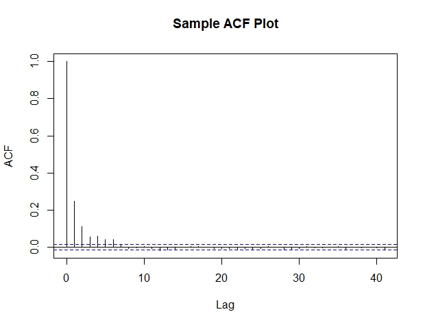
First, we can look at the autocorrelation function of the MCMC observations for our model parameters. I’ve included a sample ACF for Beta1 below. The acf plot shows that correlation quickly converges to 0, which is a good sign.

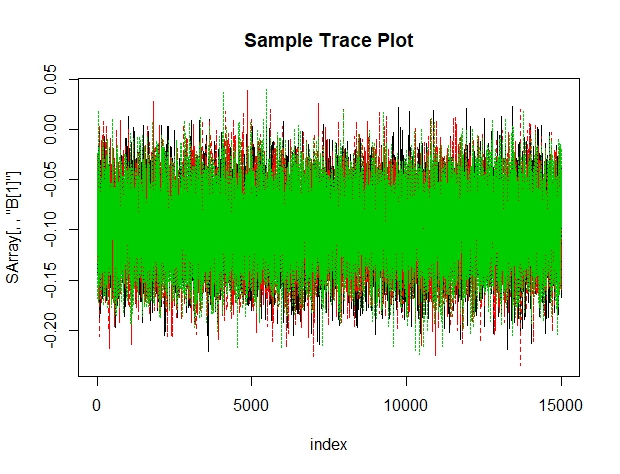
We can also take a look at the trace plots for our model parameters. Again, I’ve included the trace plot for Beta1 as a sample. It seems to be bouncing nicely around a central mass and we don’t see it still trending or converging towards a final value.

Looking at pretty pictures is fun, but we can get a little bit more formal with our convergance diagnostics too. The Geweke diagnostic uses a time-series approach by using spectral densities to estimate the sample variances, and then doing a two‐sample test of means to compare the mean at the start of a chain with a portion closer to the end. This let’s us know if our chain has been burned in enough.

SArray = housing.sim$sims.array
geweke.diag(SArray[,,"B[1]"], frac1=0.1, frac2=0.5)

#output
Fraction in 1st window = 0.1
Fraction in 2nd window = 0.5 

   var1    var2    var3 
 0.4808 -0.1968 -0.2762

With a large enough number of iterations, the T-test can be approximated by the standard normal. We see that the absolute value of the z-scores for all chains is less than 1.96. This means we can treat the first 10% of the data as burn-in.

We can also use the Gelman–Rubin convergence diagnostic to compare the estimated variances between chains and within chains for each model parameter. If these variances are drastically different, then we may not have converged and should probably run the model for more iterations.

housingcoda.sim <- bugs(bug.dat, inits, model.file = "C:\\Users\\Viktor\\Desktop\\BostonModel.txt",
                    params, n.chains=3, n.iter=20000, n.burnin=5000, n.thin=3, codaPkg = TRUE)
                    
housing.coda <- read.bugs(housingcoda.sim)

gelman.diag(housing.coda, confidence = 0.95, transform=FALSE, autoburnin=FALSE,
            multivariate=TRUE)
            
gelman.plot(housing.coda)

#output
Potential scale reduction factors:

         Point est.     Upper C.I.
B[1]              1       1.00
B[2]              1       1.00
B[3]              1       1.01
B[4]              1       1.00
B[5]              1       1.01
B[6]              1       1.01
B[7]              1       1.00
B[8]              1       1.00
B[9]              1       1.01
B[10]             1       1.01
B[11]             1       1.00
B[12]             1       1.00
B[13]             1       1.01
B[14]             1       1.01
deviance          1       1.00
tau               1       1.00

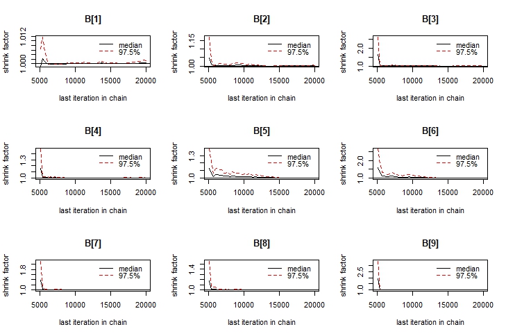
We see that all of our shrink factors are either 1 or very close to 1, and the plots show visible evidence of convergance as well.

Results:

Now that we’ve convinced ourselves that the MCMC has converged properly, we can take a look at the posterior distributions for our model parameters to determine what factors impacted house prices.

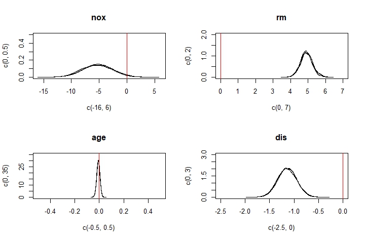
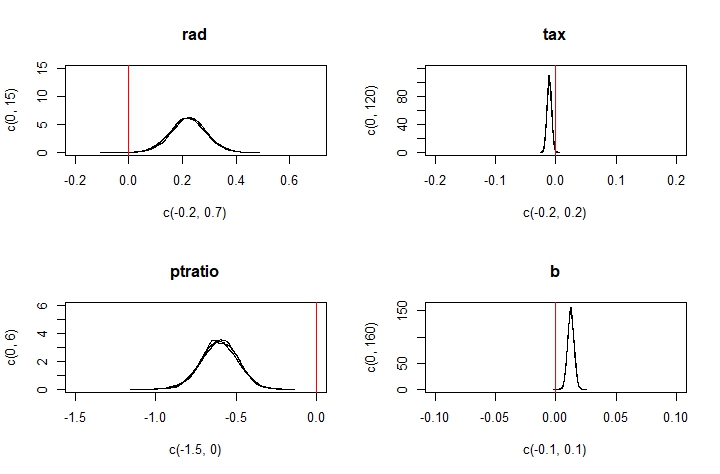
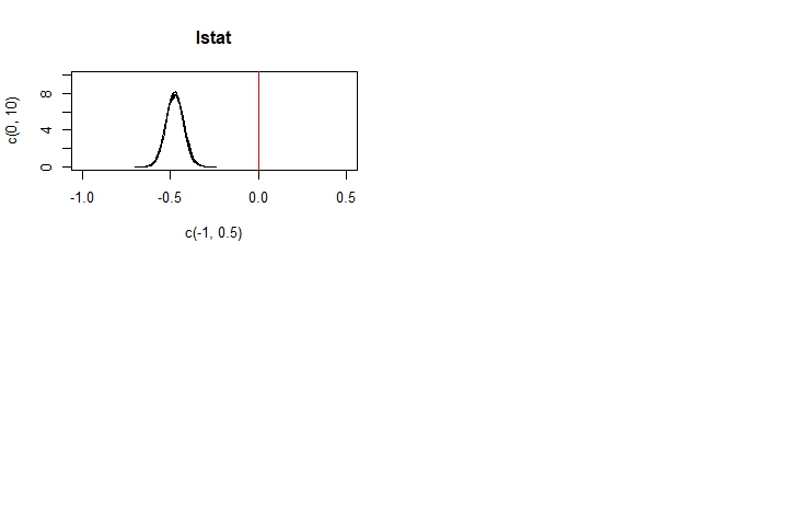
We can see that the rm, dis, ptratio, and lstat variables all have parameters that differ greatly from 0. These tell us that for our data, houses with more rooms command higher prices, and houses further from major employment centres, houses in areas with lower pupil-to-teacher ratios, and houses in lower-status areas cost less.

Intuitively, these results make sense. Holding other factors constant, a bigger house (one with more rooms) should cost more. Being further from employment centres and being in lower-status areas both provide dis-utility, and so houses with these characteristics must be discounted appropriately. Having more pupils for each teacher means each student gets less attention, which is undesirable. Do people really factor student-teacher ratios that heavily into their home purchasing decisions though? Maybe, maybe not. It may be the case that public schools (which may be more likely to exist in less well-off areas) have worse pupil-teacher ratios than expensive private schools (that may be more common in wealthy areas). Pupil-teacher ratio would then be a proxy for neighbourhood incomes, which could also explain our findings here.

Seems like we’ve found some pretty good indicators and determinants of house prices (at least at the micro level)!