
Predicting NHL Player Salaries
Objective:
Perhaps one of the most important factors to an NHL team’s success, both on and off the ice, is in its allocation of money towards individual player contracts. In terms of on-ice performance, a successful team must not only maximize the quality of its players, but do so against the NHL’s team salary cap constraint. The salary cap is a hard cap on the upper limit of each individual team’s player payroll, and is currently set at US$79.5 million. Awarding overly generous contracts to some players therefore jeopardizes a teams’ chance at success, as there will be less money available to sign other talented players.
A player’s worth is therefore a crucial piece of information for a NHL team as it will determine the optimal size of contract that each player should be awarded; unfortunately, a players’ exact worth is often quite subjective, and always difficult to ascertain. Let’s see if we can use machine learning techniques to predict player salaries based on player characteristics and performance measures from the 2016-2017 NHL season.
Analysis:
Load the required packages and the data, which is from http://www.hockeyabstract.com
I’ve already done a little bit of data cleaning in Excel (removing extra titles/headings, formatting, etc) to make the dataset more readable by R.
library(mlbench)
library(caret)
library(glmnet)
library(neuralnet)
library(party)

setwd("C:\\Users\\Viktor\\Desktop")
dat = read.csv("NHL_2016-17_Cleaned.csv", header = T)
dat = na.omit(dat)
There are 153 columns in our dataset, so we have lots of variables to analyze for our 873 players who played at least one NHL game that season. Unforunately, many of these variables will not be useful. We can start off by removing any categorical variables with too many categories (like city of birth and team) as well as variables that we know shouldn’t factor into salaries (like first and last name). We can also remove variables that are perfectly or highly correlated (like time on ice in seconds and time on ice in minutes).
After narrowing down our dataset a little bit, we can take a look at the summary stats for some of the key variables left over to give us an idea of what we’re going to be working with.
subdat = dat[,c(1,5,6,12:14,17:20,24,27,36,38,42,50,57,145,152)]
sumstat = sapply(subdat, mean)

sumstat = data.frame("Statistic" = colnames(subdat),
                     "Mean" = sapply(subdat, mean),
                     "Median" = sapply(subdat, median),
                     "Standard Deviation" = sapply(subdat, sd),
                     "Minimum" = sapply(subdat, min),
                     "Maximum" = sapply(subdat, max))
sumstat
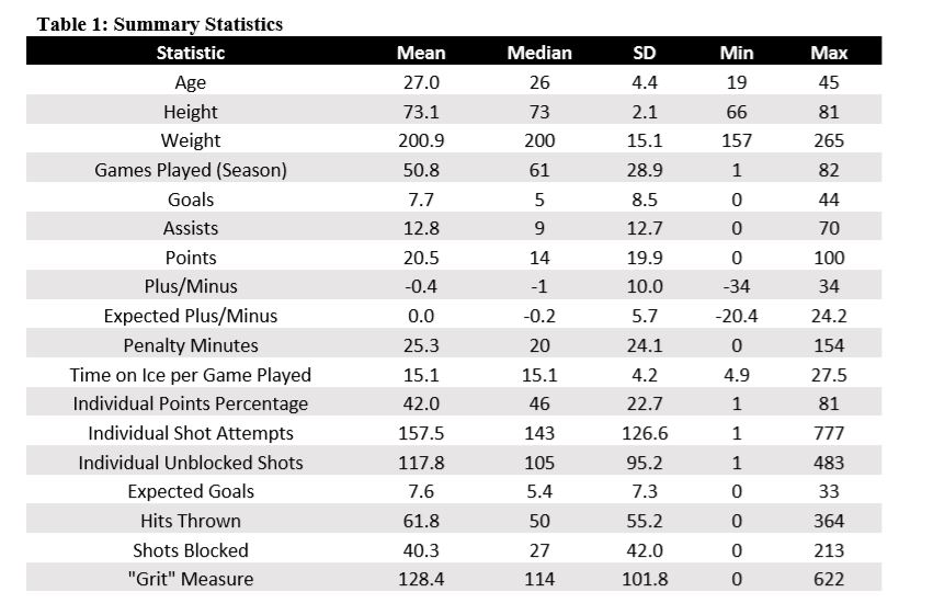
The salary variable, which is what we’ll try to predict, is each player’s salary in USD in the 2016-2017 NHL season. It ranged from a low of $575,000 to a high of $14,000,000 with a mean of $2,351,415 and a median of $950,000.
To prevent overfitting, we’ll likely need to cut down the number of features in our model a bit further. We can use recursive feature elimination for this.
#Divide into training and test sets
set.seed(42)
idx = createDataPartition(subdat$Salary, p = 0.8, list = FALSE)
dat_trn = subdat[idx, ]
dat_tst = subdat[-idx, ]

# do feature selection using a random forest selection function
control <- rfeControl(functions=rfFuncs, method="cv", number=5)
results <- rfe(dat_trn[,c(1:18)], dat_trn[,19],
               sizes=c(1:10), rfeControl=control)
print(results)
# the chosen features
predictors(results)
plot(results, type=c("g", "o"))
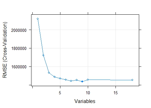
The random forest RFE revealed that RMSE was minimized when nine variables were included in the model. The nine chosen variables were: age, time on ice per game played, individual shot attempts, individual unblocked shots, assists, points, shots blocked, games played, and expected goals.
With the optimal number of variables determined, we can now centre and scale our data and feed these features into some predictive models. Let’s test out six different models, just for fun to see how they stack up against each other for this dataset. We would probably get slightly better results if we determined the optimal subset of features for each different model individually rather than using the same set from our RFE for each one, but using the same inputs for each will save a lot of time and make our lives much easier.
#Create subset of dataset using the optimal selection of features
dat_trn = dat_trn[,c(19, 1, 11, 6, 4, 14, 13, 7, 15, 17)]
dat_tst = dat_tst[,c(19, 1, 11, 6, 4, 14, 13, 7, 15, 17)]

# centre and scale inputs, which will matter for some of our models
dat_trn$Age <- scales::rescale(dat_trn$Age, to=c(0,1))
dat_trn$TOI.GP <- scales::rescale(dat_trn$TOI.GP, to=c(0,1))
dat_trn$A <- scales::rescale(dat_trn$A, to=c(0,1))
dat_trn$iCF <- scales::rescale(dat_trn$iCF, to=c(0,1))
dat_trn$iFF <- scales::rescale(dat_trn$iFF, to=c(0,1))
dat_trn$PTS <- scales::rescale(dat_trn$PTS, to=c(0,1))
dat_trn$iBLK <- scales::rescale(dat_trn$iBLK, to=c(0,1))
dat_trn$GP <- scales::rescale(dat_trn$GP, to=c(0,1))
dat_trn$ixG <- scales::rescale(dat_trn$ixG, to=c(0,1))

dat_tst$Age <- scales::rescale(dat_tst$Age, to=c(0,1))
dat_tst$TOI.GP <- scales::rescale(dat_tst$TOI.GP, to=c(0,1))
dat_tst$A <- scales::rescale(dat_tst$A, to=c(0,1))
dat_tst$iCF <- scales::rescale(dat_tst$iCF, to=c(0,1))
dat_tst$iFF <- scales::rescale(dat_tst$iFF, to=c(0,1))
dat_tst$PTS <- scales::rescale(dat_tst$PTS, to=c(0,1))
dat_tst$iBLK <- scales::rescale(dat_tst$iBLK, to=c(0,1))
dat_tst$GP <- scales::rescale(dat_tst$GP, to=c(0,1))
dat_tst$ixG <- scales::rescale(dat_tst$ixG, to=c(0,1))

x_train = dat_trn[,c(2:10)]
x_test = dat_tst[,c(2:10)]

y_train = dat_trn[,c(1)]
y_test = dat_tst[,c(1)]
We’ll use cross-validation to train most of our models, except for the random forest which will use out-of-bag error (OOB will give the same result, it’s just faster).
cv_5 = trainControl(method = "cv", number = 5)
oob = trainControl(method = "oob", number = 5)
The first two models we’ll use will be support vector regressions (SVR), which is a variation of the support vector machine (SVM) training algorithm. A SVM is a binary linear classifier that seeks to draw a line that separates the points of two different categories in feature space. Nonlinear models can also be created using the kernel trick, which involves the use of a non-linear kernel function to transform data into a higher-dimensional feature space, where classes will then be linearly separable.
Let’s use one SVR with a linear kernel and a second SVR using the kernel trick and a radial basis function kernel to see how they compare.
linGrid = expand.grid(C = c(2^ (-5:5)))
SVM_Lin = train(x_train, y_train,
                method="svmLinear", tuneGrid= linGrid,
                trControl = cv_5)
SVM_Lin
sqrt((mean((predict(SVM_Lin, x_test) - y_test)^2)))


radGrid = expand.grid(sigma= 2^c(-25, -20, -15,-10, -5, 0), C= 2^c(0:5))
SVM_Rad = train(x_train, y_train,
                method="svmRadial", tuneGrid= radGrid,
                trControl = cv_5)
SVM_Rad
sqrt((mean((predict(SVM_Rad, x_test) - y_test)^2)))
The optimal value of our cost “C” in our linear kernel SVM during 5-fold CV was determined to be C=1. For the Radial Basis Function Kernel we found optimal values of sigma = 0.03125 and C = 8.
Next, let’s use a k-nearest neighbours model. This is a non-parametric method that, in the case of regression, predicts an output for a point by averaging the values of the k points nearest to the point of interest in feature space. Distance for a KNN model in feature space is generally calculated using Euclidian distances, but other distance metrics can be used as well. A number of different values for k can be fed into the model, and during training the value that provides the most accurate predictions can be learned and used later in testing.
k_set = data.frame(k=c(1, 3, 5, 7, 9, 11, 13, 15, 17, 19, 21, 23, 25))
knn = train(x_train, y_train,
            method="knn", tuneGrid= k_set,
            trControl = cv_5)
knn
sqrt((mean((predict(knn, x_test) - y_test)^2)))
The final value used for the KNN model was k = 9.
Now let’s train a random forest, which is an ensemble model that involves bootstrap aggregating (bagging) a multitude of decision trees to reduce variance. Random forests include a random element to the selection of model features, as only a random subset of all available features are selected as candidates during any split.
rf = train(x_train, y_train,
            method="rf", trControl = oob)
rf
sqrt((mean((predict(rf, x_test) - y_test)^2)))
The final value used for the model was mtry = 5, which means that five features will be randomly sampled for potential use for each split.
Next we’ll use a Bayesian regularized neural network. Regularization adds an additional term to the loss function that the model seeks to minimize with this additional term serving as a penalty for larger model weight matrices. While simple regularizers such as weight decay can be used to limit model complexity, a Bayesian approach can also be taken by applying a Maximum A Posteriori (MAP). The MAP can be derived by employing Bayes’ Theorem to find the mode of the posterior distribution of the model weights given the training dataset, which is then converted into the cost function used in regularization.
Now, I know what you’re thinking: “Viktor, we’re only working with 873 observations here, surely a neural network is overkill and will lead to overfitting.” And you would be correct. But counterargument: neural networks are cool and Bayesian stats makes me feel trendy, so I’m going to do it anyway.
nnet = train(x_train, y_train,
              method = "brnn",
              trControl = cv_5)
nnet
sqrt((mean((predict(nnet, x_test) - y_test)^2)))
The final model selected was a two layer network with three neurons.
Finally we’ll train a boosted GLM, which involves running a large number of model iterations with a special focus being placed on data points that were not predicted well in previous iterations. Bootstrap samples of the total data are formed for each iteration of the model with points randomly selected for each sample, but in each re-sample, the probability of a specific point being selected correlates with the prediction error for that point in the previous model iteration.
glmboost = train(x_train, y_train,
              method="glmboost",
              trControl = cv_5)
glmboost
sqrt((mean((predict(glmboost, x_test) - y_test)^2)))
The model was run for 150 boosted iterations.
Results:
Now let’s compare the root mean squared error for these models to see how accurate their predictions were.
Model = c()
Model[1] = "Linear Kernel SVM"
Model[2] = "RBF Kernel SVM"
Model[3] = "KNN"
Model[4] = "Random Forest"
Model[5] = "Bayesian Regularized Neural Network"
Model[6] = "Boosted Generalized Linear Model"

CV.RMSE = c()
CV.RMSE[1] = min(SVM_Lin$results$RMSE)
CV.RMSE[2] = min(SVM_Rad$results$RMSE)
CV.RMSE[3] = min(knn$results$RMSE)
CV.RMSE[4] = min(rf$results$RMSE)
CV.RMSE[5] = min(nnet$results$RMSE)
CV.RMSE[6] = min(glmboost$results$RMSE)

TestRMSE = c()
TestRMSE[1] = sqrt((mean((predict(SVM_Lin, x_test) - y_test)^2)))
TestRMSE[2] = sqrt((mean((predict(SVM_Rad, x_test) - y_test)^2)))
TestRMSE[3] = sqrt((mean((predict(knn, x_test) - y_test)^2)))
TestRMSE[4] = sqrt((mean((predict(rf, x_test) - y_test)^2)))
TestRMSE[5] = sqrt((mean((predict(nnet, x_test) - y_test)^2)))
TestRMSE[6] = sqrt((mean((predict(glmboost, x_test) - y_test)^2)))

frame = data.frame("Model" = c(Model),
                   "CV Train RMSE" = c(CV.RMSE),
                   "Test RMSE" = c(TestRMSE))
frame
#output
                       Model               CV.Train.RMSE    Test.RMSE
1                   Linear Kernel SVM       1554538         1661133
2                      RBF Kernel SVM       1355049         1601657
3                                 KNN       1487434         1559010
4                       Random Forest       1405866         1636663
5 Bayesian Regularized Neural Network       1436819         1744622
6    Boosted Generalized Linear Model       1542204         1657226
We see that K-NN model has the lowest test RMSE. The RBF kernel SVM performs better than the linear kernel SVM, so capturing some non-linearities was useful for model prediction. The RBF kernel SVM, random forest, and BRNN all seem to show some signs of overfitting with their fairly low training errors but poor performance on held-out test data. Then the boosted GLM, like the linear kernel SVM, performs poorly in both training and testing, probably because linear models are not very suitable for this particular dataset.
So some of our models did alright, but why can’t any of them make super accurate predictions? Inaccuracies could stem from player salaries being “sticky.” Since contracts are generally awarded for multi-year periods, yet player performance can fluctuate significantly over this time, player statistics and characteristics in the current year may not be strong predictors of player salary. This would especially be the case for young players still on entry-level contracts and aging veterans in the latter half of a long contract that was signed closer to their prime. Having player performance statistics for the year of contract signing would probably help our models quite a bit.
Overall, this has been a fun little experiment on comparing models. The next installment in this NHL salary prediction series will see if we can get a little bit fancier to improve predictions using XGBoost.
Update: The next post, Revisting NHL Salary Prediction with XGBoost is up and ready to go.